The self organizing tree (SOT) is a type of artificial neural network based on the self organizing map (SOM). It uses an unsupervised, competitive learning algorithm to store representations of the input space. Unlike the conventional SOM, where a data point is given to every node of the SOM, in SOTs a forward propagation requires to compute a competition between only $log(N)$ nodes, where $N$ is the number of nodes the model has. This makes the SOT computationally significantly more efficient than a conventional SOM. The neighbourhood of a SOT is also differently defined than in a SOM. While in a 2D SOM, nodes are organized in a grid like fashion, the SOT’s nodes are organized in the form of a binary tree. The binary tree structure allows SOTs to find a best matching unit with fewer steps, however, its computational efficiency comes with a cost. While in the SOM, $N$ nodes can become best matching units, in the SOT only $N/2$ of the nodes can potentially become best matching units. In this short blog post, I’ll only explain the fundamentals of how a SOT works. Why it’s useful and how it can be used, I’ll explain in Part 2.

Introduction - Self Organizing Map

The self organizing map (SOM), also known as the Kohonen map, differs quite a lot from today’s backpropagation-based artificial neural networks. While backpropagation-based neural nets correct their weights by computing gradients according to a cost function, nodes in SOMs update their weights through competitive learning. In competitive learning, nodes in a network compete for the right to activate for a certain input. As a result, each node specializes overtime to fire only when a specific input is given. This specialization of nodes caused by competition, can also be viewed as a variant of Hebbian learning.

To prevent confusion, when learning about SOMs, it’s best to forget anything you know about neural networks. There are no activation functions, no backpropagation, no dot product between inputs and weights. The architecture of a (2D) SOM simply consists of a grid of neurons (also known as units, or nodes). Each node of the SOM is fully connected to the input layer, as shown in figure 1.

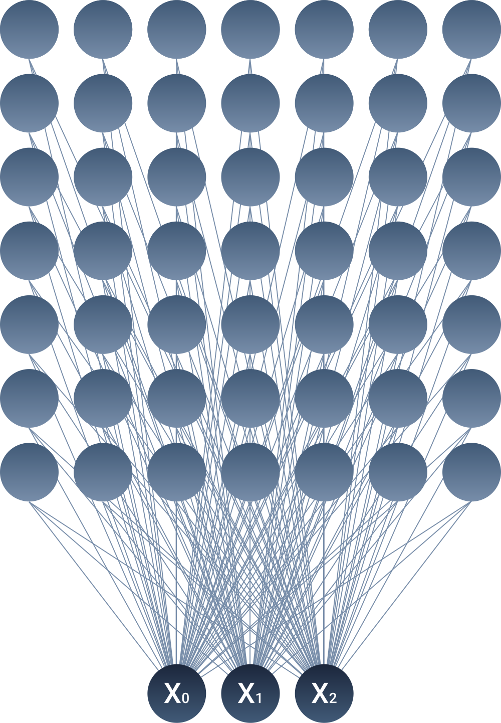
Figure 1. Illustration of a SOM architecture.

As SOMs are trained in an unsupervised way, no targets are necessary to train it. After the weights of the model are initialized, competitive learning is used during training. The steps of the learning algorithm are straightforward:

• Compute the Euclidean distance of the input vector and the weight vectors of the SOM.
• Find the node with the smallest distance. This node is also called the best matching unit (BMU).
• The BMU neighbourhood radius is calculated. The neighbourhood radius usually starts as a large value and gradually decreases with every time step (Note: There are SOM variants where the neighbourhood radius does not decrease according to the time step, allowing for online learning without a pre-defined number of iterations).
• The weight vector of every node inside this neighbourhood radius is adjusted to become more similar to the input vector. The further away a node is from the BMU, the less its weights are updated.
• Repeat all steps for N iterations.

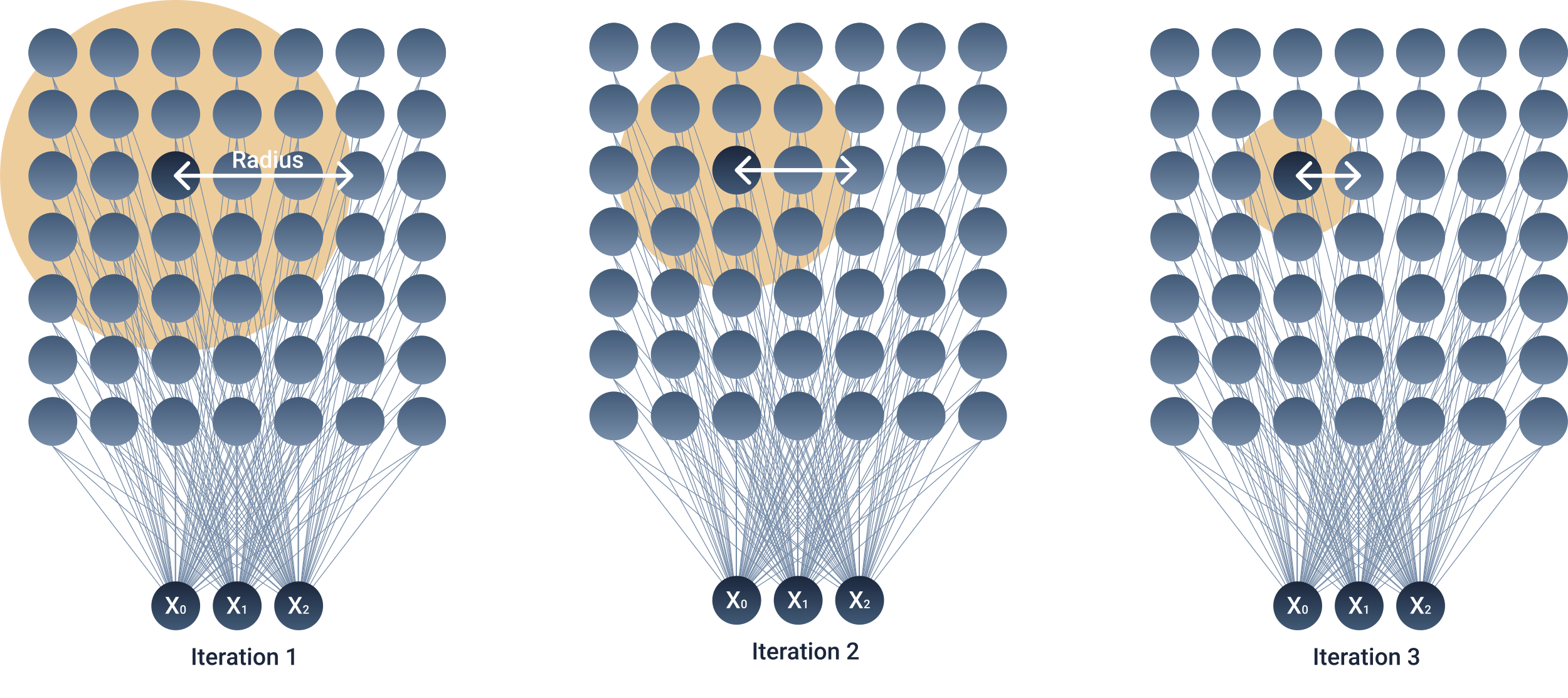
Figure 2. Illustration of the SOM's neighbourhood radius changing with every iteration.

Because of the competitive learning algorithm, SOMs are able to preserve the topological properties of the input space, allowing for nice visualizations. SOMs in fact are rarely used for anything else these days, but as we will see in future posts, the core ideas of SOMs can be quite useful. A nice SOM implementation in PyTorch can be found here. If you want to know more about the SOM implementation, AI-Junkie’s blog post goes in great depth.

Self Organizing Tree

In a SOM, we have to calculate the Euclidean distances between the input vector and all the weight vectors. For large SOMs, this can be computationally demanding. In the SOT on the other hand, we have to calculate only $2 * log(N)$ Euclidean distances, where $N$ is the number of nodes in the SOT. That is because the SOT’s architecture - it is structured as a binary tree (see figure 3).

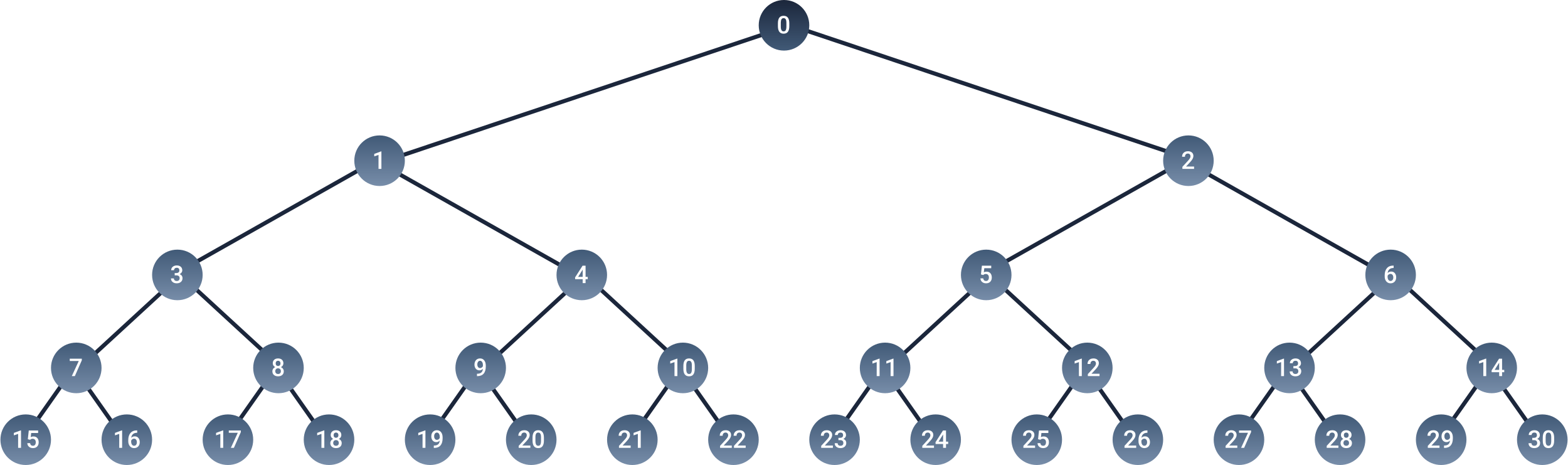
Figure 3. The architecture of a self organizing tree. Every node contains a weight vector.

Before going into how the learning algorithm of the SOT works, let’s first have a closer look at the architecture. In figure 3, I have labeled every node with an index. The indices serve just for clarification. The node with the zero index represents our input vector, or our input node. Every other node in the tree contains a weight vector that has the same size as the input vector. The nodes of the tree that do not have any children, are also known as leaf nodes. In contrast to SOMs, where every node can potentially become the BMU for an input, in the SOT only leaf nodes can become BMUs. The intermediate nodes in the tree, i.e. the ones that have children, are known as Non-leaf nodes, or simply as parent nodes. The number of layers per tree is also known as the tree depth (denoted as $D$). A tree with 16 leaf nodes for example, will have a depth of 4.

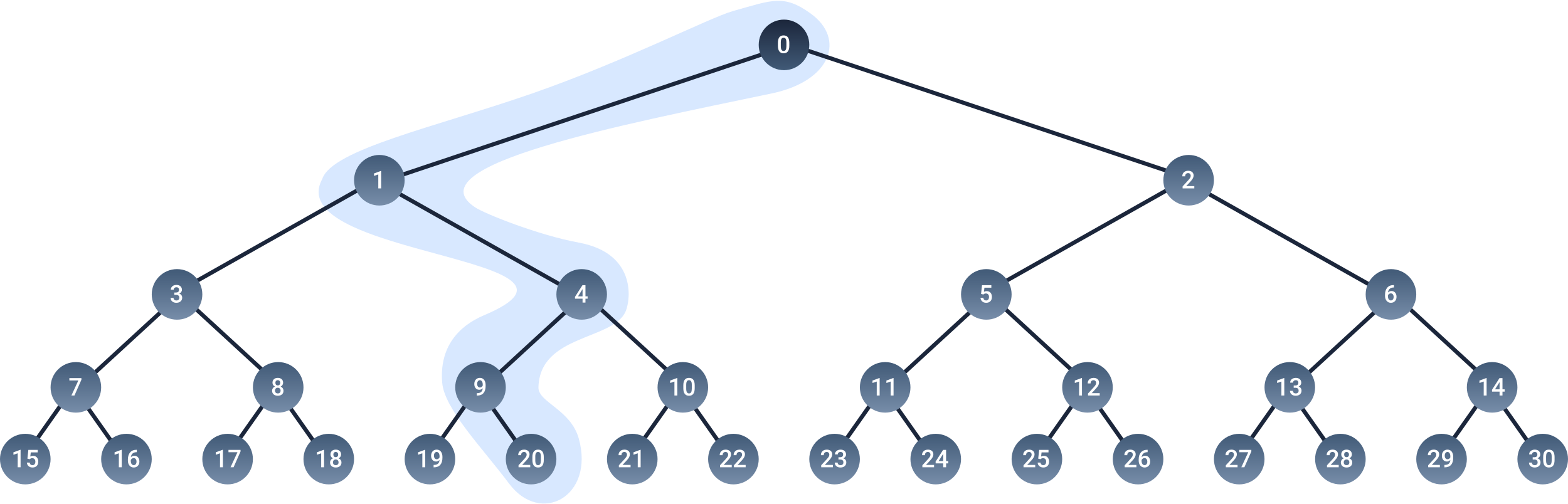
Figure 4. An input vector propagating through the self organizing tree. The nodes inside the blue line, represent the nodes that won the layer-wise competitions.

When training a SOT, instead of feeding the input vector to every single node in the tree, we simply feed it to the children of the input layer (nodes $1$ and $2$). We then compute the Euclidean distance for the two nodes. The node that wins the competition, i.e. the node with the smallest distance, feeds the input vector to its children. The competition repeats until two leaf nodes are reached (see figure 4). As we can see, in the SOT, only two nodes compete with one another per layer. After $D$ iterations, the input vector will have passed through the tree and will have reached two leaf nodes, where the last competition is calculated. The winning leaf node represents the BMU.

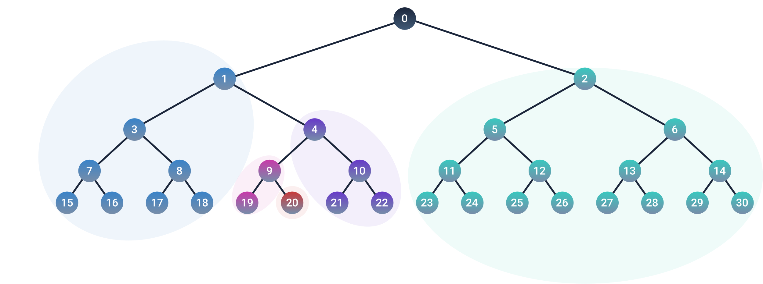
Figure 5. An illustration showing how nodes in a tree are updated in clusters. The BMU (node 20) is updated the most. Its parent node and its other branch get updated slightly less. The parent node of the parent node, and its other branch get updated even less, and so on. The learning rate diminishes the further away we get from the BMU in the tree.

After finding the BMU for a given input vector, the weight vector of every node is adjusted to become more similar to the input vector (see figure 5). The learning rates for the updates are “tree-depth-dependent”. We will have $D$ learning rates, ordered in decreasing order. The BMU is updated with the largest learning rate, adjusting it closer to the input vector. When we go one level up the tree (to the BMU’s parent node), the parent node and its other branch will be updated with the second learning rate, which is slightly smaller than the BMU’s learning rate. The higher we go up the tree, the less every branch and parent gets updated. An implementation of the self organizing tree can be found in this Github repository.

After some iterations, the nodes of the SOT will specialize to fire to specific inputs. The code below is an example of how to train a simple SOT with 32 leaf nodes on the fashion-mnist dataset.

from torchvision import datasets, transforms
from torch.utils.data import DataLoader
from SOT import SOT
import torch

transform = transforms.ToTensor()
training_set = datasets.FashionMNIST("~/.pytorch/F_MNIST_data", download = False, train = True, transform = transform)
train_dataloader = DataLoader(training_set,  
                            shuffle = True,  
                            batch_size = 1,  
                            num_workers = 0  
                            )

# initialize self organizing tree
device = torch.device('cpu')
tree = SOT(number_of_leaves = 32,
                input_dim = 28*28,
                lr = 0.2,
                device = device
               )

iterations = 10000
num = 0
for data in train_dataloader:
    x, y = data
    bmu = tree.forward(x.flatten())
    num += 1
    if num >= iterations:
        break

After a few iterations, patterns will start to emerge in the weight vectors of the SOT (see figure 6). SOTs have an interesting attribute: The further away we go from the leaf nodes, i.e. the closer we get to the input node, the less meaningful the weights get (see figure 7). The first two nodes of the SOT are basically just blobs. The deeper we get in the tree however, the more specialized the nodes will be.

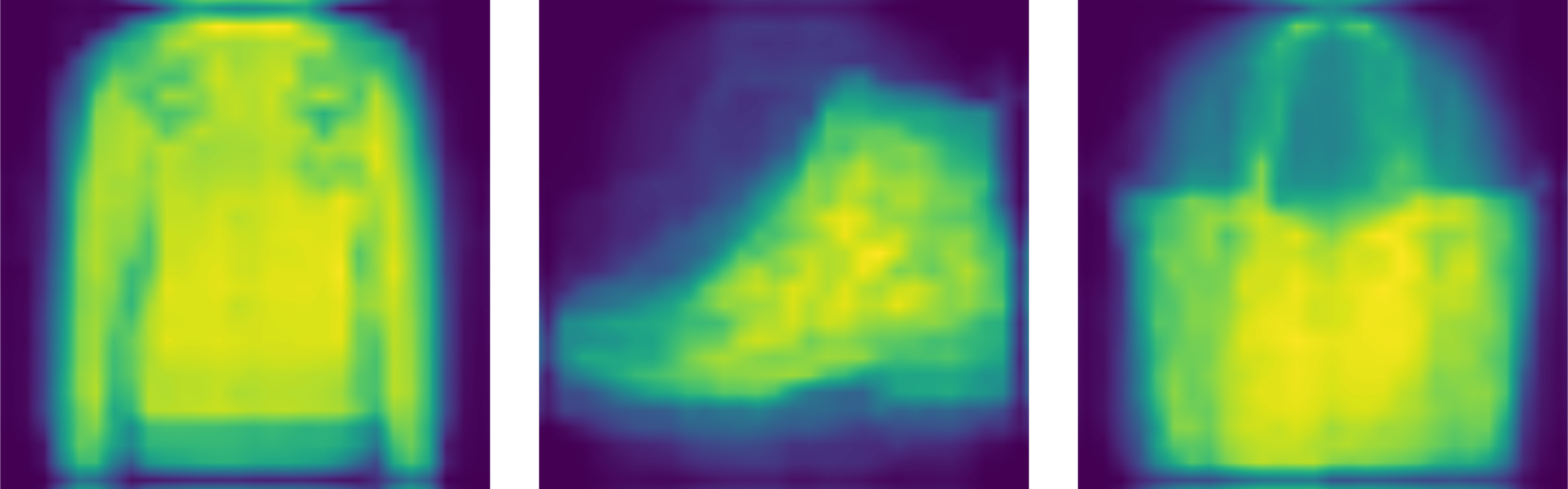
Figure 6. The weight vectors of three leaf nodes taken from from the SOT that was trained on the fashion-mnist dataset. Darker regions represent weight values close to zero, whereas lighter regions represent weight values closer to one. Leaf nodes are the most specialized nodes in the SOT.

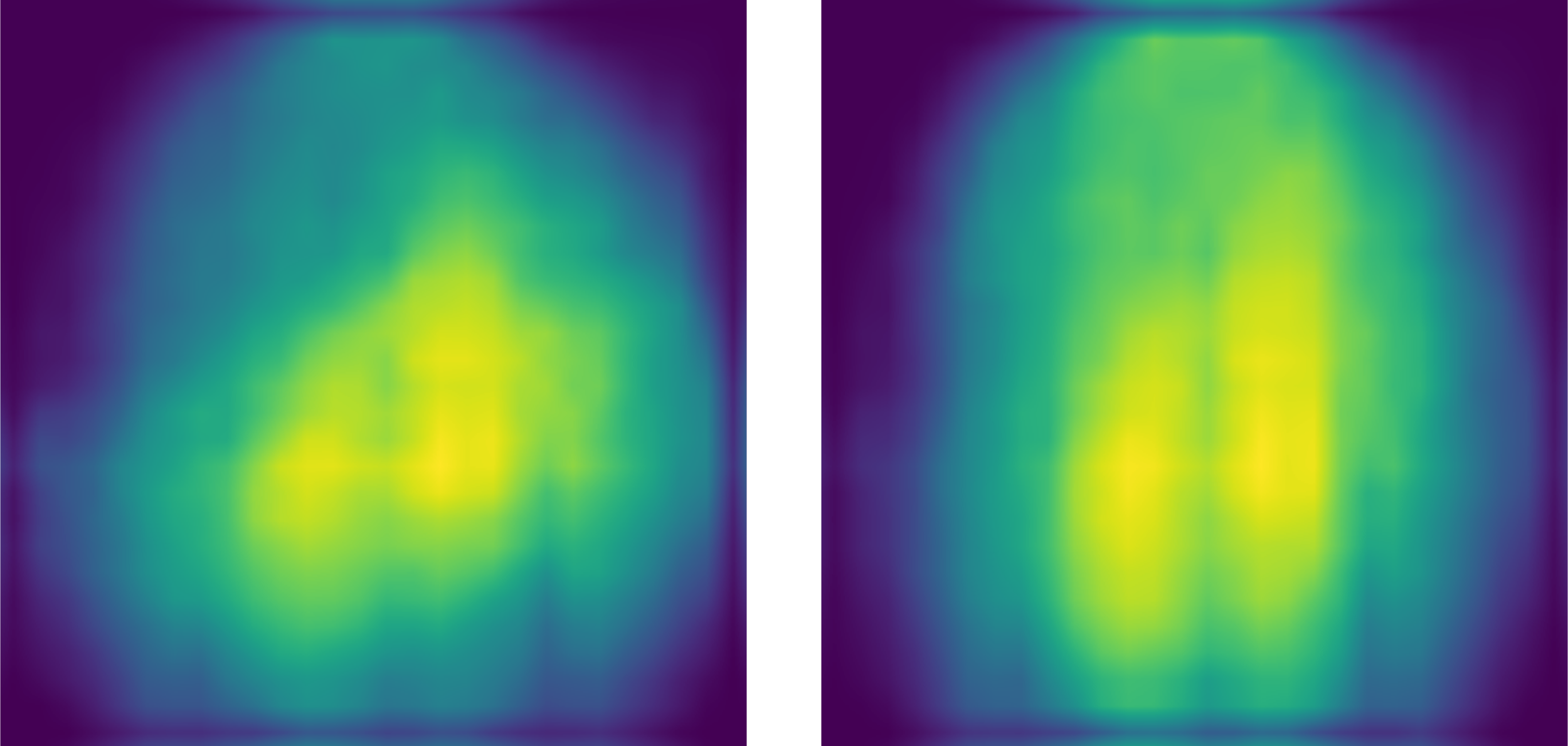
Figure 7. The weight vectors of the first two nodes of the SOT. Darker regions represent weight values close to zero, whereas lighter regions represent weight values closer to one. The first nodes are the least specialized nodes in the SOT.

The necessary lack of specialization of the non-leaf nodes that are close to the input node, can be problematic when performing a forward pass. If for some reason a wrong turn is taken during propagation, the input vectors can end up landing at the wrong leaf node and mess up the state of the already specialized nodes. Logically, the more possible states an input vector can have, the more likely it gets for an input vector to make a mistake during propagation, compared to a case where we have less possible states. To better understand the problem, Lets take an example (see figure 8 as a reference): Lets say a certain input vector, $X_a$, usually gets mapped at node $29$, or at a leaf node close to $29$. This region of the tree is specialized to fire whenever it sees $X_a$. Now lets say another input $X_b$ propagates through the tree and lands at leaf node $24$. If this happens often enough, the weight vector at node $2$ might change just about enough so that next time $X_a$ appears, instead of taking the path through node $2$, it propagates through node $1$ and lands at node $20$, which was already specialized for another pattern.

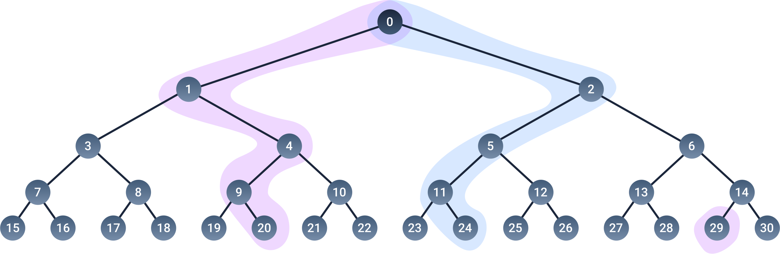
Figure 8. An illustration how a "path" through the tree can overtime get erased by other input vector, causing input vectors to land at the wrong leaf nodes.

This flaw is a dealbreaker. Having a self organizing map variant that requires only $log(N)$ competitions is great, but not if it means sacrificing the ability to preserve the topological properties of the input space. Not everything might be lost however. If the input vectors are not too large, and the patterns that can occur are not too numerous, such erasures might not have to occur at all. Lets see how that works.

Convolutional Self Organizing tree

You can find an implementation of a 2D convolutional self organizing tree (ConvSOT) here. The ConvSOT simply combines the idea of convolutional neural networks (CNN) with the SOT. Before feeding the input vector to the model, we divide it into overlapping local image patches of size $z \times z$, where $z$ is the kernel size. Instead of having the internal weights of the SOT as large as the whole input vector itself, the weights of each node are also only $z \times z$ in size. Inside the SOT, each patch of the input propagates through the tree in parallel.

Figure 9. Illustration of how an input gets fed to the convolutional self organizing tree. Each input gets divided into overlapping patches of size z x z, which then get fed in parallel to the tree.

The weight vectors of the SOT then get updated by taking the mean of the weight adjustments for each input patch. Since the kernel sizes are relatively small compared to the input vector, the possible shapes that we will find in these patches is also relatively small. This alone should be enough to prevent path erasures in the tree and keep the topology preserving property of regular SOMs. And this is exactly what we will see when training such a tree (see figure 10): Overtime the tree will learn various basic shapes in the different branches of the tree.

Figure 10. Illustration of the internal weight vectors of a trained convolutional self organizing tree.

The output of the ConvSOT layer will be a $L\times K$ matrix of leaf node indices, where $L$ represents the number of image patches in the rows of the input matrix, and $K$ represents the number of patches in the columns of the input matrix. As you can probably already notice, We could stack additional convolutional self organizing tree “layers” on top of the first layer, feeding the output of one layer to the next. We could do that, though I will not do that here. But for those who want to code this capability, it’s important to note that after the first hidden layer, the next layers cannot use the Euclidean distance for the competitions. I might clarify this in a future post.

Great, now we know how a convolutional self organizing tree works, but how does one use them? Or more exactly, why would one want to use SOTs in the first place? In Part 2 of this blog series, I’ll explain how we can combine the self organizng tree with autoencoders, and build something really cool and useful :)